Lemma 3.15. (Vitali type covering lemma. ) Let  be a collection of open balls in
  , and let
  . If
. If  , there exist disjoint
  such that
Proof. The set  is open, then for
  there exists a compact set
  such that
 .
.
Since is compact, there exists finitely many balls  such that
  . Let
. Let  be the collection of the balls. Choose
  that has the largest radius. Let
  be the collection of balls from
  that is disjoint from
  . Choose the ball
  that has the largest radius. In general, suppose that
  are choosen. Let
  be the collection of balls in
  that are disjoint from the previous
  balls
balls  . Choose
  that has the largest radius. Since there are only
  balls, the process will stop. We assume that
  are the finally chosen balls. Given any ball
  , we claim that
  will intersect with some ball from
  . Otherwise, one more ball will be chosen. A contradiction. Hence
So  .
.
Definition. A measurable function  is called locally integrable with respect to the Lebesgue measure if
  for every bounded measurable set
  The space of such functions is denoted by
Definition. If  , we define
 .
.
Lemma 3.16. If  ,
,  is jointly continuous in
  .
.
Proof. Given  . Since ,
  . By Corollary 3.6, given
  , there exists
  such that if
  ,
,

So given , if  ,
,
 .
.
So  So
So
Hence as ,

Definition. If , the Hardy-Littlewood maximal function  by
by

Remark. The function is measurable for

is open for any  .
.
Theorem 3.17. There is a constant  such that for any
  and
and  ,
,
 .
.
Proof. Let  . For
. For  , there exists
  such that
 .
.
Let  . For any , by Vitali type lemma 3.15, there exists disjoint balls
  ,
,

Note that the right hand side does not depend on  . Let
. Let  , we prove that
This proves Theorem 3.17.
We shall use the notion of limit superior for real valued functions of a real variable.

So  is equivalent to
Theorem 3.18. If , then  .
.
Proof. Since we are investigating continuity of a funtion at a point, it is a local property. So we may assume that . Secondly, it is easy to see that the claim is true for a continuous function.
Now given , there exists a continuous function  such that
  Consider


Hence 
Given any ,

By the maximal theorem,

Let  , we see that
  . We rationalize
  , we see that

Definition. For any , define the Lebesgue set  of
of  to be
to be
 .
.
Theorem. If , then 
Proof. For any  ,
,  . Then for
  ,
,

Let  . Then
For any  , there exists
  such that
  ,
,

So 
Let  ,
,

Thus  . Since
  ,
, 
Definition. A Borel measure  is called “
regular" if (i).  for every compact . (ii).
  , for any
  . A signed measure or complex measure is called
 “regular” if  is regular.
Theorem 3.22. Let be a regular signed or complex Borel measure on , and  be its Lebesgue-Radon-Nikodym representation. Then for
  ,
,
 .
.
Proof. We make two observations. (i). If is regular, so are  . (ii). We may assume that
  , because
  .
.
We know that  are mutually singular. Let
  be a Borel set such that
  Let
Let
 . We will show that
  for all , which will complete the proof with the aid of the Lebesgue-Radon-Nikodym theorem.
By the regularity of , for any , there exists open set  such that
  and
and  For any
  , there exists
  such that
  . Let
. Let  and
and  , there exists
  and disjoint balls
  such that


Let  . We see that
  . Since
  ,
,  . So
. So 
Theorem 3.23. Let  be increasing, and let
  .
.
(a). The set of points at which  is discontinuous is countable.
(b). and  are differentiable
  , and
, and 
Proof. (a). Let  . It is clear that is the set of points at which is discontinuous. Since
  is increasing, for
  ,
,

Also for  , the interval
  contains a rational number. So is at most countable.
(b). We observe that is increasing and right continous.  except perhaps where is discontinuous. Moreover
![G(x+h)-G(x) = \begin{cases} \mu_G((x,x+h]), \text{ if }h>0, \\ -\mu_G((x+h,x]), \text{ if }h<0\end{cases}.](https://s0.wp.com/latex.php?latex=G%28x%2Bh%29-G%28x%29+%3D+%5Cbegin%7Bcases%7D+%5Cmu_G%28%28x%2Cx%2Bh%5D%29%2C+%5Ctext%7B+if+%7Dh%3E0%2C+%5C%5C+-%5Cmu_G%28%28x%2Bh%2Cx%5D%29%2C+%5Ctext%7B+if+%7Dh%3C0%5Cend%7Bcases%7D.+&bg=ffffff&fg=4b5d67&s=0&c=20201002)
We know that  is regular. So by Theorem 3.22,
  exists .
Let  . We need to show that
  exists and equals zero Let
  be an enumeration of points at which
  , i.e.,
  . Given any
  ,
,

Let  . Then
  is a Borel measure that is finite on compact sets by
  . Then is a Lebesgue-Stieltjes measure.
We know that
 . This goes to zero as
  for by Theorem 3.22. Indeed, let
  . Then
  since
since  is at most countable;
  . So
. So  . Thus exists , and
Definition. If  and
and  , we define

 is called the total variation of $F$.
Remark. It is easy to observe that for $a<b$,

Thus is an increasing function with values in ![[0,\infty]](https://s0.wp.com/latex.php?latex=%5B0%2C%5Cinfty%5D&bg=ffffff&fg=4b5d67&s=0&c=20201002) .
.
Definition. (1). If  , is said to be of bounded variation on
  . We denote the space of all such functions by
  .
.
(2). The supremum in is called the total variation of on ![[a,b]](https://s0.wp.com/latex.php?latex=%5Ba%2Cb%5D&bg=ffffff&fg=4b5d67&s=0&c=20201002) . If it is finite, then we say that
. If it is finite, then we say that ![F\in BV([a,b])](https://s0.wp.com/latex.php?latex=F%5Cin+BV%28%5Ba%2Cb%5D%29&bg=ffffff&fg=4b5d67&s=0&c=20201002) .
.
Examples. (1). If  is bounded and increasing, then
(2). If  and
and  , then
(3). If is differentiable on and  is bounded, then . Hint: using the mean value theorem.
(4). If  , then for
  , but
, but  One can see it by taking
  .
.
(5). If  for
for  and
and  , then
 ![F\notin BV([a,b])](https://s0.wp.com/latex.php?latex=F%5Cnotin+BV%28%5Ba%2Cb%5D%29&bg=ffffff&fg=4b5d67&s=0&c=20201002) for
for  . One can see it by taking
  .
.
Lemma 3.26. If  and is bounded, then
  is increasing.
Proof. If , then by ,
 .
.
Theorem 3.27. (1). iff  .
.
(2). If , then iff is the difference of two bounded increasing functions. For the  direction, we take
  .
.
(3). If , then  exist for all . This follows from (1) and (2).
(4). If , the set of points at which is discontinuous is countable. This follows from (1) and (2).
(5). If and  , then
  exist and are equal a.e. This follows from (1), (2) and Theorem 3.23.
Definition. NBV=\{F\in BV:\, F \text{ is right continuous and } F(-\infty) =0\}.
Remark. If , then the function defined by  is in NBV and
  . Indeed, ; so
  the difference of two increasing functions.
  is again the difference of two increasing functions. So
  .
.  is obvious.
Theorem 3.28. If , then  . If is also right continuous, so is .
Proof. Given and , then by the definition of , there exists  such that

So by ,
 . This proves that
  Since is increasing,
  for all
  . So .
For the second claim, we define  and assume that . For any , since $F$ is right continuous and
  is defined, there exists such that for
  ,
,

For any such  , there exists
  such that
 , and so

Similarly on the interval ![[x,x_1]](https://s0.wp.com/latex.php?latex=%5Bx%2Cx_1%5D&bg=ffffff&fg=4b5d67&s=0&c=20201002) , we apply the same reasoning to conclude that there exists
, we apply the same reasoning to conclude that there exists  so that
 .
.
So on ![[x, x+h]](https://s0.wp.com/latex.php?latex=%5Bx%2C+x%2Bh%5D&bg=ffffff&fg=4b5d67&s=0&c=20201002) ,
,

On the other hand, 
So that  . Since
  is arbitrary, a contradiction. Therefore
  .
.
Theorem 3.29. If is a complex measure on and ![F(x) = \mu((-\infty, x])](https://s0.wp.com/latex.php?latex=F%28x%29+%3D+%5Cmu%28%28-%5Cinfty%2C+x%5D%29&bg=ffffff&fg=4b5d67&s=0&c=20201002) , then
, then  . Conversely if , there is a unique complex Borel measure
  such that
 ![F(x) = \mu_F((-\infty, x])](https://s0.wp.com/latex.php?latex=F%28x%29+%3D+%5Cmu_F%28%28-%5Cinfty%2C+x%5D%29&bg=ffffff&fg=4b5d67&s=0&c=20201002) ; moreover
; moreover  .
.
Proof. Suppose that is a complex measure. By decomposing into real and complex parts, and then considering the positive and negative parts of measures,
 . Since is a complex measure,
  are finite positive measures. Let
 ![F_j^\pm = \mu^\pm_j ((-\infty,x])](https://s0.wp.com/latex.php?latex=F_j%5E%5Cpm+%3D+%5Cmu%5E%5Cpm_j+%28%28-%5Cinfty%2Cx%5D%29&bg=ffffff&fg=4b5d67&s=0&c=20201002) . Then
. Then  are right continuous, increasing functions. Also
  and
and  . By Theorem 3.27 (1) and (2),
Conversely, for , we write  by Theorem 3.27 (1) and (2). Then by Theorem 3.27, each
  is bounded and increasing. Then
  . By Theorem 3.28, is right continuous and so $T_F$ is right continuous. So each
  is right continuous by Theorem 3.28. Also it is easy to see that each by Theorem 3.28 again. So by Theorem 1.16,
 ![F_j^\pm(x)= \mu_{F_j^\pm}((-\infty, x])](https://s0.wp.com/latex.php?latex=F_j%5E%5Cpm%28x%29%3D+%5Cmu_%7BF_j%5E%5Cpm%7D%28%28-%5Cinfty%2C+x%5D%29&bg=ffffff&fg=4b5d67&s=0&c=20201002) for some finite Borel measure
for some finite Borel measure  . Let
. Let  .
.
The last step is to show that . It is contained in Exercise 28 and 21 in Folland’s book.
Theorem 3.30. If , then  . Morevoer
  iff
iff  , and
, and  iff
iff 
Proof. Since , then $\mu_F$ in Theorem 3.29 is a complex Borel measure that is also regular. Then by the Radon-Nikodym theorem,
 , where
  , where
 ![E_r=(x,x+r], \text{ or } (x-r, x]](https://s0.wp.com/latex.php?latex=E_r%3D%28x%2Cx%2Br%5D%2C+%5Ctext%7B+or+%7D+%28x-r%2C+x%5D&bg=ffffff&fg=4b5d67&s=0&c=20201002) by Theorem 3.22. The rest conclusions follows easily from the Radon-Nikodym representation above.
by Theorem 3.22. The rest conclusions follows easily from the Radon-Nikodym representation above.
Proposition 3.32. If , then is absolutely continuous iff .
Proof.  If , then by Theorem 3.5, we see that the claim holds.
 We need to prove that for
  , if , then
  . Since is absolutely continuous, then for any , there exists such that for any finite disjoint intervals
  , then if
  ,
,
Since , there exists a sequence of open sets  such that
  ,
,  latex \mu_F$ is regular, we can find a sequence of open sets
  such that
  such that
  . That is to say,
  as
as  . Therefore
  is a sequence of open sets that are decreasing and contains , and moreover
  . We abbreviate it by .
Each is an at most countable union of disjoint open intervals  . For any
  ,
,

So  Since
Since  , we see that
 Since is arbitrary,
  .
.
Corollary 3.33. If  , then the function
  is in NBV and is absolutely continuous, and
  Conversely if is absolutely continuous, then and
  .
.
Proof. Suppose that . Then  , right continuous and
  by dominated convergence theorem. So
  That is absolutely continuous follows from Corollary 3.6. By Theorem 3.32, the deduced measure and also
  .
.  by Theorem 3.30. On the other hand,
  gives rise to the same function . By the uniqueness in Theorem 3.29, $fdm$ and $F’dm$ are the same complex Borel measures. Hence
Conversely, if and is absolutely continuous, then by Theorem 3.32. Hence by Theorem 3.30,  Considering the real and imaginary parts of complex valued functions, and positive and negative parts of real-valued functions, we see that
  because is a complex Borel measure.
Lemma 2.34 If is absolutely continuous on , then .
Proof. We know that is absolutely continuous. Let be given. There exists such that for disjoint intervals  with
with  , then

Let $N$ be the smallest integer that is larger than  . We divide into consecutive segments with length that is at most
  . For any points
  , if necessary adding more endpoints of the previous consecutive segments , so that these points can be grouped into subgroups. On each subgroup, if the points are denoted by
  ,
,  So the total sum is majorized by
  This holds true for any partition of . So .
Theorem 3.35 (The fundamental theorem of calculus for Lebesgue integrals.) If and ![F:[a,b]\to \mathbb{C}](https://s0.wp.com/latex.php?latex=F%3A%5Ba%2Cb%5D%5Cto+%5Cmathbb%7BC%7D&bg=ffffff&fg=4b5d67&s=0&c=20201002) , the following are equivalent:
, the following are equivalent:
(a) is absolutely continuous on $[a,b]$
(b)  for some
 ![f\in L^1([a,b], m)](https://s0.wp.com/latex.php?latex=f%5Cin+L%5E1%28%5Ba%2Cb%5D%2C+m%29&bg=ffffff&fg=4b5d67&s=0&c=20201002) .
.
(c) is differentiable on , ![F'\in L^1([a,b], m)](https://s0.wp.com/latex.php?latex=F%27%5Cin+L%5E1%28%5Ba%2Cb%5D%2C+m%29&bg=ffffff&fg=4b5d67&s=0&c=20201002) , and
, and  .
.
Proof.  By subtracting
  and extending to trivially, we may assume that by Lemma 3.34. So by Corollary 3.33,
  follows.
 is trival.
 Extending trivially to , i.e.,
 ![f(t)=0, t\notin [a,b]](https://s0.wp.com/latex.php?latex=f%28t%29%3D0%2C+t%5Cnotin+%5Ba%2Cb%5D&bg=ffffff&fg=4b5d67&s=0&c=20201002) . Then we invoke Corollary 3.33.
. Then we invoke Corollary 3.33.


![\nu((a,b]) = \lambda_f(a)-\lambda_f(b)](https://s0.wp.com/latex.php?latex=%5Cnu%28%28a%2Cb%5D%29+%3D+%5Clambda_f%28a%29-%5Clambda_f%28b%29&bg=ffffff&fg=4b5d67&s=0&c=20201002)
![\phi=1_{(a,b]}](https://s0.wp.com/latex.php?latex=%5Cphi%3D1_%7B%28a%2Cb%5D%7D&bg=ffffff&fg=4b5d67&s=0&c=20201002)

![RHS = -\int_a^b d\lambda_f = \nu((a,b]) = \lambda_f(a)-\lambda_f(b)](https://s0.wp.com/latex.php?latex=RHS+%3D+-%5Cint_a%5Eb+d%5Clambda_f+%3D+%5Cnu%28%28a%2Cb%5D%29+%3D+%5Clambda_f%28a%29-%5Clambda_f%28b%29&bg=ffffff&fg=4b5d67&s=0&c=20201002)


![[f]_p = \left( \sup_{\alpha>0} \alpha^p \lambda_f(\alpha)\right)^{1/p}.](https://s0.wp.com/latex.php?latex=%5Bf%5D_p+%3D+%5Cleft%28+%5Csup_%7B%5Calpha%3E0%7D+%5Calpha%5Ep+%5Clambda_f%28%5Calpha%29%5Cright%29%5E%7B1%2Fp%7D.+&bg=ffffff&fg=4b5d67&s=0&c=20201002)

![\{f:\, f \text{ is measurable and } [f]_p<\infty\}.](https://s0.wp.com/latex.php?latex=%5C%7Bf%3A%5C%2C+f+%5Ctext%7B+is+measurable+and+%7D+%5Bf%5D_p%3C%5Cinfty%5C%7D.+&bg=ffffff&fg=4b5d67&s=0&c=20201002)

![[\cdot]_p](https://s0.wp.com/latex.php?latex=%5B%5Ccdot%5D_p&bg=ffffff&fg=4b5d67&s=0&c=20201002)


![[f]_2= \sup_{\alpha}\alpha^2 \lambda_f(\alpha)=1.](https://s0.wp.com/latex.php?latex=%5Bf%5D_2%3D+%5Csup_%7B%5Calpha%7D%5Calpha%5E2+%5Clambda_f%28%5Calpha%29%3D1.+&bg=ffffff&fg=4b5d67&s=0&c=20201002)


![[f+g]_2 =4.](https://s0.wp.com/latex.php?latex=%5Bf%2Bg%5D_2+%3D4.+&bg=ffffff&fg=4b5d67&s=0&c=20201002)
 The
The  When
When  Define
 . Indeed, there exists
  such that
  . Then
  . Since the latter sets are increasing,
  .
.  ,
,  is a vector space. Indeed,
  . Then
  .
.  .
.  is a normed vector space.
  iff
iff  and for any
  . It remains to prove the triangle inequality, i.e.,
  .
. ![p \in [1,\infty]](https://s0.wp.com/latex.php?latex=p+%5Cin+%5B1%2C%5Cinfty%5D&bg=ffffff&fg=4b5d67&s=0&c=20201002) and
and  is the conjugate exponent such that
  Then
Then  .
.  for some
  .
.  . For
. For  ,
,  .
.  ,
,  This proves the triangle inequality.
  and
and  ,
,  Equality holds iff
  .
.  for
for  . Then by the geometric observation the rectangle with side lengths
  has an area less than the sum of two areas under
  with respect to the
  axises.
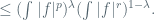
  . Let
. Let  . Then
  . Integration on both sides gives
 . On the other hand, we know that
  . Therefore
 That the equality holds iff
  .
.  be a Cauchy sequence in
  such that
 .
.  by the monotone convergence theorem. Then for
  . Let
. Let  be the measure zero set associated with
  because
  .
.  converges to
  in
in  Then
Then  Then by the dominated convergence theorem,

 , where
  , is dense in
  , then
  .
.  , let
, let  . Then
 and
and 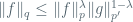 , where
  such that
  .
. 
 . Define
 is a linear functional on
 .
.  are conjugate exponent and
  . If
. If 
 and
and  , define
  .
. 

 Then
Then  . So if
  such that
  . Let
. Let 
 . So
. So
 for all
  of simple functions that vanish outside a set of finite measure, and the quantity
 is
is  .
. 
 such that
 pointwise. Since
  and
and  by assumptions, then the dominated convergence theorem yields
 is
is  be an increasing sequence of sets of finite measure such that
 pointwise. Let
  . Then
 pointwise and
  vanishes outside
  . Let
. Let 
 . By Fatou’s lemma,

 , so the proof is complete for the case
  .
. . Given
  If
If 
 .
.  there exists
  for all
  is isometrically isomorphic to
  . The same conclusion holds for
  finite.
  .
. , if
, if  , we have that
  .
.  converges in the
  as $n\to \infty$.
 . So
. So  . So
. So  . By the Radon-Nikodym theorem, there exists
  such that
  for all
  for all simple functions
  . So
. So  with increasing
  such that for all
  ,
, 

 on
on  . We define
  . Then
  is the increasing limit of
  . Moreover,
  in
in 
 is a map
  such that
  .
.  , then
 .
.  converges absolutely. That is to say,
 . One can prove that
  are signed measures. The total variations
  are bounds for
  .
.  ,
,  .
.  are complex measures, we say that
  if
if  for $a, b= r, i.$ If
  is a positive measure, we say that
  if
if  and
and  .
.  such that
  and
and  If also
  and
and  , then
  and
and  .
.  and
and  ,
, , an extended
  . We know that at most one of
  and
and  is infinite. Suppose that
  , we will obtain a contradiction to that
  measurable. Since
  are mutually singular, there exist a disjoint decomposition of
  , such that
  and
and 
 .
. . The same applies to
  ,
,  and
and  . Thus
  .
.  . Let
. Let  . It is easy to verify that that is the desired decomposition.
  where
where  .
.  for a finite measure
  . Then Theorem 3.12 can be applied to obtain the existence of
  let
let  , then by Proposition 3.9,
 Since
Since  is nonnegative, we see that
  ,
,
 . Take
  and
and  , where
  are the Hahn decomposition for
  So the new definition of the total variation agrees with the old definition.
  for all
  .
.  and
and  has absolute value
 and if
  .
.  , where
 .
.  . Then
  by Theorem 3.12 and
  .
. ,
, 

 ,
,  Let
Let  . Then
  Thus
Thus 
 are complex measures on
  .
. ![\nu: \mathcal{M}\to [-\infty, \infty]](https://s0.wp.com/latex.php?latex=%5Cnu%3A+%5Cmathcal%7BM%7D%5Cto+%5B-%5Cinfty%2C+%5Cinfty%5D&bg=ffffff&fg=4b5d67&s=0&c=20201002) such that
such that 
 .
. 
 are measures on
  is a signed measure. Indeed, Let
  be a sequence of disjoint sets in
  and
and  ,
, 
 is a signed measure. The case where one of them is infinite is proved similarly.
  be a measure space; let
 ![f:X\to [-\infty, \infty]](https://s0.wp.com/latex.php?latex=f%3AX%5Cto+%5B-%5Cinfty%2C+%5Cinfty%5D&bg=ffffff&fg=4b5d67&s=0&c=20201002) is a measurable function such that at least one of
is a measurable function such that at least one of  is finite, then
  is a signed measure. Indeed, for
  ,
,  is a measure on
  . If
. If  .
.  disjoint, then
 , where
  It is easy to see that
  is disjoint.
 .
.  If
If  is finite, then we have continuity from above.
 . A set $E$ is called positive for
  , then
  . Similarly for negative sets and null sets.
 ![f:\, X\to [-\infty, \infty]](https://s0.wp.com/latex.php?latex=f%3A%5C%2C+X%5Cto+%5B-%5Cinfty%2C+%5Cinfty%5D&bg=ffffff&fg=4b5d67&s=0&c=20201002) be a measurable function. Let
be a measurable function. Let  , for
, for  on
on  If there exists
  with
with  , but
, but  . We derive a contradiction. Writing
 ,
,  such that
  . Call this set
  . Then
  . Then
  A contradiction.
  be a sequence of positive sets. The proof follows by writing
  as a disjoint union.
  and a negative set
  and
and  . If $P’, N’$ is another such pair, then
  is null for
  . Two observations.
  and
and  . Thus
  . This applies to any measurable subset of
  .
.  . Let
. Let 
 . If setting
  . We may assume that
  is increasing. Then
 is negative.
  with
with  . We claim that there exists
  . Otherwise one can show that
  such that
  . By (ii), there exists
  satisfying
  . Let
. Let  be the pair such that
  and
and 

 is attained. Let
  be the corresponding set. Suppose that
  are chosen.
 . Then
 . Obviously we have


 , there exists
  . Thus there exists
  such that
 .
.  of
of  such that
  ,
,  . Informally speaking, ”
 such that
  and
and 
 For any
 ;
;  . Thus
  .
.  . The new measures
  live on different sets
  respectively. It is not hard to show that
  is positive for
  is negative for
  is null for
  ,
,  latex \mu^ \nu(E\cap N_1)$ also equals the previous sum. Also
  . Thus
  . Likewise,
  .
.  are called the positive and negative variations of
  is called the Jordan decomposition of
  .
.  .
.  is equivalent to
  is equivalent to

 .
.  if
if  for every
  is equivalent to
 .
.  ,
,  .
.  Suppose the contrary. For
  , for any
  , there exists
  ,
,  . Let
. Let  . Then
  is decreasing and
  . Then
  because
  . Then because
  . However since
  . A contradiction.
  Let
Let  be given as above. For
  This is true for any
  . Hence
 ![f\to [-\infty, \infty]](https://s0.wp.com/latex.php?latex=f%5Cto+%5B-%5Cinfty%2C+%5Cinfty%5D&bg=ffffff&fg=4b5d67&s=0&c=20201002) is a measurable function such that at least one of
is a measurable function such that at least one of  is finite. In this case, we shall call
  . Then
 and
and  .
. 
 is equivalent to
 and
and  on
on  be a Hahn decomposition for
  , and let
  and
and  . Then for all
  . Since
  is a finite measure,
  .
.  , then
  , there for some
  ; therefore
  is a positive set for
  on
on  and
and  .
.  such that
  , and any two such functions are equal a.e.
 ![\mathcal{F} =\{f:\, X\to [0,\infty] \text{ is measurable } \int_E fd\mu \le \nu(E) \text{ for all } E\in \mathcal{M}\}](https://s0.wp.com/latex.php?latex=%5Cmathcal%7BF%7D+%3D%5C%7Bf%3A%5C%2C+X%5Cto+%5B0%2C%5Cinfty%5D+%5Ctext%7B+is+measurable+%7D+%5Cint_E+fd%5Cmu+%5Cle+%5Cnu%28E%29+%5Ctext%7B+for+all+%7D+E%5Cin+%5Cmathcal%7BM%7D%5C%7D&bg=ffffff&fg=4b5d67&s=0&c=20201002) .
.  because
  .
.  . Then
  . There exists a sequence of
  , such that
  . Let
. Let  . Then
  . Aso
. Aso  is increasing. Let
  . By the monotone convergence theorem,
 . Then
 . That is to say,
  . Let
. Let  . Then
  . However
  . A contradiction.
  . Then
 .
. ,
,  . Thus
  and therefore
  . This implies
  . Similarly
  . Next we need to prve the uniqueness of
  .
.  and
and  . So
. So  such that
  . Thus $g=g_1, a.e.$.
  ,
,  and
and  are disjoint. Let
  . Then
  such that
  and
and  such that
  . Let
. Let  , where
  . Let
. Let  . One can verify that
  and
and  . Indeed, by definition,
  . For
. For  and for each
  , there exists a Hahn decomposition
  satisfying that
  , and
, and  live on
  . Then
  . We verify that
  live on
  respectively: for each
  and for each
  , then
  This proves that
  ,
,  on
on  on
on  is
is 
 .
.  . Then one can verify that
  and
and  Indeed, if
  . Then
 is the Hahn decomposition for
  such that
  respectively. So
 . Thus
  and
and  . A contradiction to the definition of
  . Take
  . Then
  . Therefore
  because part (1) and part (2) apply to
  Therefore
  with
with  is called the Lebesgue decomposition of
  be as above and
  . In this case,
  is called the Radon-Nikodym derivative of
  .
.  are
are  .
.  , then
  and
and  .
. 
 . For
. For  .
.  holds true for
  . Then by usual procedure, it is true for
  follows from the equation by considering
  and
and  . This proves (a).
  . Note that the equation in (a) does not require
 and
and  , then
  (with respect to either
  , there exists a sequence
  , both are dyadic numbers, so that
  decreasing to
  and
and  increasing to
  . Thus
  , an invertible linear transform from
  . If
. If  .
.  , then
  and
and  .
.  is an invertible linear transform and so it is continuous. Therefore if
  denote the three elementary linear transforms.
  and
and 
 It is easy to see that the integration formula (*) is true for the three linear transforms because any invertible linear transforms can be written as a product of the three linear transforms. Now we check the integration formula (*) is true for
  These are the consequences of Fubini’s theorem. Indeed, for
  , we interchange the order of integration of
  and
and  . For
. For  we integrate first with the
  .
.  .
.  in (a).
  by using (b). Then the general result follows by approximations.
  defined by
  where
where  and
and  . It is easy to see that
  is a continuous bijection.
  , define
 ,
,  .
.  on
on  ,
,  on
on  such that
  . If
. If 

 .
.  is clear.
  . For
. For ![(a,b]\times B](https://s0.wp.com/latex.php?latex=%28a%2Cb%5D%5Ctimes+B&bg=ffffff&fg=4b5d67&s=0&c=20201002) , where
, where ![\rho \times \sigma ((a, b]\times B) = \rho((a,b]) \sigma(B) = \frac {b^n-a^n}{n} \sigma(B)](https://s0.wp.com/latex.php?latex=%5Crho+%5Ctimes+%5Csigma+%28%28a%2C+b%5D%5Ctimes+B%29+%3D+%5Crho%28%28a%2Cb%5D%29+%5Csigma%28B%29+%3D+%5Cfrac+%7Bb%5En-a%5En%7D%7Bn%7D+%5Csigma%28B%29&bg=ffffff&fg=4b5d67&s=0&c=20201002) .
. ![(a,b]\times B= (0,b]\times B\setminus (0,a]\times B](https://s0.wp.com/latex.php?latex=%28a%2Cb%5D%5Ctimes+B%3D+%280%2Cb%5D%5Ctimes+B%5Csetminus+%280%2Ca%5D%5Ctimes+B&bg=ffffff&fg=4b5d67&s=0&c=20201002) and
and ![(0,a]](https://s0.wp.com/latex.php?latex=%280%2Ca%5D&bg=ffffff&fg=4b5d67&s=0&c=20201002) . Let
. Let ![E_a= \Phi^{-1} ( (0,a]\times B)](https://s0.wp.com/latex.php?latex=E_a%3D+%5CPhi%5E%7B-1%7D+%28+%280%2Ca%5D%5Ctimes+B%29&bg=ffffff&fg=4b5d67&s=0&c=20201002) and
and ![E_b= \Phi^{-1}((0,b]\times B)](https://s0.wp.com/latex.php?latex=E_b%3D+%5CPhi%5E%7B-1%7D%28%280%2Cb%5D%5Ctimes+B%29&bg=ffffff&fg=4b5d67&s=0&c=20201002)
![m_* ((a,b]\times B)= m(E_b\setminus E_a) =m(E_b)-m(E_a).](https://s0.wp.com/latex.php?latex=m_%2A+%28%28a%2Cb%5D%5Ctimes+B%29%3D+m%28E_b%5Csetminus+E_a%29+%3Dm%28E_b%29-m%28E_a%29.+&bg=ffffff&fg=4b5d67&s=0&c=20201002)
![m(E_a) = a^n m(\Phi^{-1} ((0,1]\times B))](https://s0.wp.com/latex.php?latex=m%28E_a%29+%3D+a%5En+m%28%5CPhi%5E%7B-1%7D+%28%280%2C1%5D%5Ctimes+B%29%29+&bg=ffffff&fg=4b5d67&s=0&c=20201002) .
.![m_* ((a,b]\times B) = \frac {b^n-a^n}{n} \sigma(B)](https://s0.wp.com/latex.php?latex=m_%2A+%28%28a%2Cb%5D%5Ctimes+B%29+%3D+%5Cfrac+%7Bb%5En-a%5En%7D%7Bn%7D+%5Csigma%28B%29&bg=ffffff&fg=4b5d67&s=0&c=20201002) .
.  on
on  and let
  be the collection of finite disjoint unions of sets of the form
 ![(a,b]\times E](https://s0.wp.com/latex.php?latex=%28a%2Cb%5D%5Ctimes+E&bg=ffffff&fg=4b5d67&s=0&c=20201002) . We know that
. We know that  both agree on
  on
on  is generated by
  both also agree on it. Next we know that
  is the set of all the Borel measurable rectangles on
  all agree on this union, so another application of the uniqueness theorem shows that
  agree on the Borel sets of
  be measure spaces. We have discussed the product
  on
on  .
.  with
with  and
and  .
.  of finite disjoint unions of rectangles is an algebra.
  .
.  .
.  .
.  . Then
  .
.  and
and  ,
,  .
.
 .
.  yields
 .
.  is the disjoint union of rectangles
  , then

 is well defined on
  , disjoint.
  ,
,  .
.  .
. 
 .
.  .
.  are
are  with
with  , then
 .
.  be a product space. If
  , for
, for  , we define the
  and the
  section
  of
of  .
. section and the
  .
.  .
.  , then
  for all
  for all
  is
is  measurable for all
  is
is  with
with  ,
, 
 , if $x\in \cap_{j} A_j$ for
  , then
 , then
  So
So  .
. 
 .
.  , then
  , we see that
  .
.  , if
, if  , then
  . This proves
 .
.  are both measurable. The proof is similar for complex valued functions.
  that is closed under countable increasing unions and countable decreasing intersections. That is to say, if
  and
and  , then
  . Likewise for intersections.
  , there is a unique smallest monotone class containing
  , namely, the intersection of all monotone classes that contain
  because
  , we show that
  ,
,  .
.  is a monotone class. For instance, if
  and
and  and
and  is decreasing. We know that
  . Similarly for
  . So
. So  .
.  contains
  , then
  is equivalent to
  . If
. If  because
  . That is to say, for
  ,
,  . This proves the claim.
  . And for
  . Thus
  . That
  are measurable on
  , respectively, and
 ,
, 
 is measurable. This reasoning can be generalized to any element in
  . By Theorem 2.35, it suffices to prove the claim for sets in the monotone class
  and
and  and
and  is increasing,
  . Since each
  is measurable, then
  is measurable. Likewise for decreasing intersection since the measures of
  .
.  and
and  is disjoint and
  . For
. For 
 is measurable. So
  is measurable. Likewise for
  , then the functions
 respectively, and
 ![\int f d(\mu\times \nu) = \int [\int f(x,y) d\nu(y)]d\mu(x) = \int [\int f(x,y)d\mu(x)]d\nu(y). (*)](https://s0.wp.com/latex.php?latex=%5Cint+f+d%28%5Cmu%5Ctimes+%5Cnu%29+%3D+%5Cint+%5B%5Cint+f%28x%2Cy%29+d%5Cnu%28y%29%5Dd%5Cmu%28x%29+%3D+%5Cint+%5B%5Cint+f%28x%2Cy%29d%5Cmu%28x%29%5Dd%5Cnu%28y%29.+%28%2A%29&bg=ffffff&fg=4b5d67&s=0&c=20201002)
 , then
  for
for  , and
, and  for
for  , then
  are in
  respectively, and
  holds.
  simple functions on
 pointwise. Then for any
  pointwise in
  . So by monotone convergence theorem,
  .
.  , then
  , which is measurable. So
  is measurable. Likewise for
  .
.  and
and  .
.  , which converges to
 ![\int [\int f_x d\nu(y)]d\mu(x)](https://s0.wp.com/latex.php?latex=%5Cint+%5B%5Cint+f_x+d%5Cnu%28y%29%5Dd%5Cmu%28x%29+&bg=ffffff&fg=4b5d67&s=0&c=20201002) . Hence we have
. Hence we have ![\int fd(\mu\times \nu=\int [\int f_x d\nu(y)]d\mu(x)](https://s0.wp.com/latex.php?latex=%5Cint+fd%28%5Cmu%5Ctimes+%5Cnu%3D%5Cint+%5B%5Cint+f_x+d%5Cnu%28y%29%5Dd%5Cmu%28x%29&bg=ffffff&fg=4b5d67&s=0&c=20201002) .
. ![\int fd(\mu\times \nu=\int [\int f^y d\mu(x)]d\nu(y)](https://s0.wp.com/latex.php?latex=%5Cint+fd%28%5Cmu%5Ctimes+%5Cnu%3D%5Cint+%5B%5Cint+f%5Ey+d%5Cmu%28x%29%5Dd%5Cnu%28y%29&bg=ffffff&fg=4b5d67&s=0&c=20201002) .
. . Then by Step 1 and 2,
 ![\int f^+ d(\mu\times \nu) = \int_X [\int_Y f_x^+d\nu(y)]d\mu(x)<\infty](https://s0.wp.com/latex.php?latex=%5Cint+f%5E%2B+d%28%5Cmu%5Ctimes+%5Cnu%29+%3D+%5Cint_X+%5B%5Cint_Y+f_x%5E%2Bd%5Cnu%28y%29%5Dd%5Cmu%28x%29%3C%5Cinfty&bg=ffffff&fg=4b5d67&s=0&c=20201002) .
.  . Thus for
  . Similarly for
  . Thus for
  ; and
; and  is an
is an  defined function and is in
  . The similar claim holds for
  with
with  . By Step 3, for
  ; moreover
  is an
is an  as
as  , and convergence in measure (to be defined).
![f_n= n^{-1} 1_{[0,n]}](https://s0.wp.com/latex.php?latex=f_n%3D+n%5E%7B-1%7D+1_%7B%5B0%2Cn%5D%7D&bg=ffffff&fg=4b5d67&s=0&c=20201002) .
. ![f_n= 1_{[n,n+1]}](https://s0.wp.com/latex.php?latex=f_n%3D+1_%7B%5Bn%2Cn%2B1%5D%7D&bg=ffffff&fg=4b5d67&s=0&c=20201002) .
. ![f_n = n1_{[0,\frac 1n]}](https://s0.wp.com/latex.php?latex=f_n+%3D+n1_%7B%5B0%2C%5Cfrac+1n%5D%7D&bg=ffffff&fg=4b5d67&s=0&c=20201002) .
. ![f_1=1_{[0,1]}](https://s0.wp.com/latex.php?latex=f_1%3D1_%7B%5B0%2C1%5D%7D+&bg=ffffff&fg=4b5d67&s=0&c=20201002) .
.![f_2= 1_{[0,\frac 12]}, f_3 = 1_{[\frac 12, 1]}](https://s0.wp.com/latex.php?latex=f_2%3D+1_%7B%5B0%2C%5Cfrac+12%5D%7D%2C+f_3+%3D+1_%7B%5B%5Cfrac+12%2C+1%5D%7D&bg=ffffff&fg=4b5d67&s=0&c=20201002) .
. ![f_4=1_{[0,\frac 14]}, f_5 = 1_{[\frac 14, \frac 12]}, f_6= 1_{[\frac 12, \frac 34]}, f_4 = 1_{[\frac 34, 1]}](https://s0.wp.com/latex.php?latex=f_4%3D1_%7B%5B0%2C%5Cfrac+14%5D%7D%2C+f_5+%3D+1_%7B%5B%5Cfrac+14%2C+%5Cfrac+12%5D%7D%2C+f_6%3D+1_%7B%5B%5Cfrac+12%2C+%5Cfrac+34%5D%7D%2C+f_4+%3D+1_%7B%5B%5Cfrac+34%2C+1%5D%7D&bg=ffffff&fg=4b5d67&s=0&c=20201002) .
. ![f_n= 1_{[\frac {j}{2^k}, \frac {j+1}{2^k}]},](https://s0.wp.com/latex.php?latex=f_n%3D+1_%7B%5B%5Cfrac+%7Bj%7D%7B2%5Ek%7D%2C+%5Cfrac+%7Bj%2B1%7D%7B2%5Ek%7D%5D%7D%2C+&bg=ffffff&fg=4b5d67&s=0&c=20201002) where
where 
 as
as  .
.  .
. 
 in measure.
  .
.  as
as 
 that converges to
  Moreover if there exists
  in measure, then
  .
. 

 has measure $0$ as
  and the sets are decreasing. On
  , there exists $n$ such that for
  ,
,  .
. 
 in measure. Indeed, given
  , on
, on  , for $l\ge k\ge n$
 .
.  . Therefore
 such that
  .
.  , and
, and  Then for any
  such that
  ,
, 
 . We denote
  .
. ,
,  on
on  .
.  , there exists
  such that
  .
.  . On
. On 
 such that for
 .
. 
 or
or  is finite, we denote
 for any
  This is easy: we distinguish three cases,
 It is to observe that, if $h = f+g,$
 . We rearrange it to obtain
  . Taking integrals on both sides yields (2).
  and
and  are both integrable.
  .
.  ,
, 


 for a.e. for all


 .
. ![f_n = \frac {1}{n} 1_{[0,n]}](https://s0.wp.com/latex.php?latex=f_n+%3D+%5Cfrac+%7B1%7D%7Bn%7D+1_%7B%5B0%2Cn%5D%7D&bg=ffffff&fg=4b5d67&s=0&c=20201002) and
and 
 such that
  If
If 

 pointwise. By DCT,
  ,
, 
 That is to say
  for
for  .
.  for each
  that is a finite unions of open intervals such that
  for some small constant
  . By taking
  , where
  is an open interval of finite length, by continuous functions
  with the following property
 . By taking
![f: X\times [a,b]\to \mathbb{C}, -\infty<a<b<\infty](https://s0.wp.com/latex.php?latex=f%3A+X%5Ctimes+%5Ba%2Cb%5D%5Cto+%5Cmathbb%7BC%7D%2C+-%5Cinfty%3Ca%3Cb%3C%5Cinfty&bg=ffffff&fg=4b5d67&s=0&c=20201002) and that
and that  is integrable for each
 ![t\in [a,b]](https://s0.wp.com/latex.php?latex=t%5Cin+%5Ba%2Cb%5D&bg=ffffff&fg=4b5d67&s=0&c=20201002) . Let
. Let  .
.  for all
  . If
. If  for every
  . In particular, if
  is continuous for each $latrex x$, then
  exists and there is a
  for all
 , the sequence of measurable functions
  is uniformly by a
![t\in [a,b], h_n\to 0](https://s0.wp.com/latex.php?latex=t%5Cin+%5Ba%2Cb%5D%2C+h_n%5Cto+0&bg=ffffff&fg=4b5d67&s=0&c=20201002) ,
, 
 , we see that the sequence
  is uniformly bounded by a
  function
  . Again by the dominated convergence theorem,

 by a partition of
 ![G_P= \sum M_j 1_{[t_{j-1}, t_j]}, g_P = \sum m_j1_{[t_{j-1}, t_j]},](https://s0.wp.com/latex.php?latex=G_P%3D+%5Csum+M_j+1_%7B%5Bt_%7Bj-1%7D%2C+t_j%5D%7D%2C+g_P+%3D+%5Csum+m_j1_%7B%5Bt_%7Bj-1%7D%2C+t_j%5D%7D%2C&bg=ffffff&fg=4b5d67&s=0&c=20201002)
 are supremum and infimum of
  whose mesh size
  and
and ![\lim_{n\to \infty} \int_{[a,b]} G_{P_n} = \lim_{n\to \infty} \int_{[a,b]} g_{P_n} = \int_{[a,b]} f (x)dx](https://s0.wp.com/latex.php?latex=%5Clim_%7Bn%5Cto+%5Cinfty%7D+%5Cint_%7B%5Ba%2Cb%5D%7D+G_%7BP_n%7D+%3D+%5Clim_%7Bn%5Cto+%5Cinfty%7D+%5Cint_%7B%5Ba%2Cb%5D%7D+g_%7BP_n%7D+%3D+%5Cint_%7B%5Ba%2Cb%5D%7D+f+%28x%29dx&bg=ffffff&fg=4b5d67&s=0&c=20201002) .
.  and
and  has the same limit.
 ![\int_{[a,b]} (G_{P_n}-g_{P_n})dx \to 0](https://s0.wp.com/latex.php?latex=%5Cint_%7B%5Ba%2Cb%5D%7D+%28G_%7BP_n%7D-g_%7BP_n%7D%29dx+%5Cto+0&bg=ffffff&fg=4b5d67&s=0&c=20201002) as
as 
![\int_{[a,b]} (G-g) dx= \lim_{n\to \infty} \int_{[a,b]} (G_{P_n} - g_{P_n}) dx](https://s0.wp.com/latex.php?latex=%5Cint_%7B%5Ba%2Cb%5D%7D+%28G-g%29+dx%3D+%5Clim_%7Bn%5Cto+%5Cinfty%7D+%5Cint_%7B%5Ba%2Cb%5D%7D+%28G_%7BP_n%7D+-+g_%7BP_n%7D%29+dx+&bg=ffffff&fg=4b5d67&s=0&c=20201002)

 pointwise,
  , which yields that
  . Since $G$ is Lebesgue measurable as simple functions and
 the space of all measurable functions from
  and
and  . We define the integral of
  .
.  .
.  , we define
 makes sense because
  .
.  be simple functions in
  .
.  ,
,  .
. 
 , then
 is a measure on
  , where
  ; so are
  . The observation is that
  takes values
  on
on  . Then
 Here we have used that
  .
.  .
. 
 ,
, 
 ,
,  Indeed, for
  , it is true. For
  we have
  . Then
  . The latter equality is because

 .
. for all
  , then
 and
and  .
.  Since
Since  and
and  such that
 . Therefore
  . Since
![f= \begin{cases} 1, x\in [-1,0)\\ -\frac 1n, x\in [0,n] \end{cases}.](https://s0.wp.com/latex.php?latex=f%3D+%5Cbegin%7Bcases%7D+1%2C+x%5Cin+%5B-1%2C0%29%5C%5C+-%5Cfrac+1n%2C+x%5Cin+%5B0%2Cn%5D+%5Cend%7Bcases%7D.+&bg=ffffff&fg=4b5d67&s=0&c=20201002)
 . It is clear that
  but
but 
![f_n(x) = 1_{[n,n+1]}](https://s0.wp.com/latex.php?latex=f_n%28x%29+%3D+1_%7B%5Bn%2Cn%2B1%5D%7D&bg=ffffff&fg=4b5d67&s=0&c=20201002) . It converges to
. It converges to  but
but 
 , then
 .
.  .
. 
 considers the set
 , because
  , then
 . A contradiction.
  .
.  ,
,  .
. 


 , then
  is a null set and
  is
is 